Using einsum for vectorizing matrix ops
An old theoretical physics course that I took introduced me to the wonders of the Einstein summation convention. I had to vectorize some matrix operations recently for multivariate normal liklihood calculations, \(X * X^T\) and \(Y * X\), on a large list of matrices (shape \((n, k, k)\)). Using einsum for this gives a massive performance boost.
import numpy as np

X = np.arange(16).reshape(4, 2, 2)
Sa = np.einsum('aij,akj->aik', X, X)

np.all([np.all(Sa[i, ...] == X[i, ...] @ X[i, ...].T) for i in range(4)])

Y = np.arange(4).reshape(2, 2)
Sb = np.einsum('ij,ajk->aik', Y, X)

np.all([np.all(Sb[i, ...] == Y @ X[i, ...]) for i in range(4)])
Efficient inverse-matrix multiplication
This uses a cholesky decomposition to calculate the inverse.
\[L^T / (L / y) = (LL^T)^{-1}y\]import numpy as np
naive = np.linalg.solve(A, b)
L = np.linalg.cholesky(A)
efficient = np.linalg.solve(L.T, np.linalg.solve(L, b))Efficient Inference of GP Covariances
Sometimes, it is easier to do parameter inference in the frequency domain. One can use SymPy (or another symbolic computation program) to get the theoretical spectrum of a GP (using a Fourier transform of the covariance function - see the Wiener-Khinchin theorem) and we use the Whittle likelihood to fit the parameters of the process using the spectrum. Similar ideas can be found in William Wilkinson’s papers and Turner and Sahani (2014).
Sampling Periodic GPs using the State Space Representation
The representation is due to Solin & Sarkka (2014).
Python Code
import numpy as np
from scipy.special import iv

"""
Adapted from matlab code from Arno Solin and Simo Sarkka (2014).
Explicit Link Between Periodic Covariance Functions and
State Space Models. Available at https://users.aalto.fi/~asolin/.

magnSigma2   : Magnitude scale parameter
lengthScale  : Distance scale parameter
period       : Length of repetition period
mlengthScale : Matern lengthScale
N            : Degree of approximation
nu           : Matern smoothness parameter
mN           : Degree of approximation if squared exonential
valid        : If false, uses Bessel functions

df(t)/dt = F f(t) + L w(t)
spectral denisty of w(t) is Qc
y_k = H f(t_k) + r_k, r_k ~ N(0, R)

"""

def reformat(conv_function):
    def wrapper(*args, **kwargs):
        F, L, Qc, H, Pinf = conv_function(*args, **kwargs)
        if len(L.shape) == 1: L = np.diag(L)
        if len(H.shape) == 1: H = H.reshape(1, -1)
        if type(Qc) is not np.ndarray: Qc = np.array(Qc).reshape(1, 1)
        if len(Qc.shape) == 2: Qc = np.diag(Qc)
        return F, L, Qc, H, Pinf
    return wrapper

class StateSpaceModels:

    @staticmethod
    @reformat
    def Periodic(magnSigma2 = 1, lengthScale = 1, period = 1, N = 6):

        q2 = 2 * magnSigma2 * np.exp(-1/lengthScale**2) *\
            iv(np.arange(0, N + 1), 1/lengthScale**2)
        q2[0] *= 0.5

        w0 = 2*np.pi/period
        F = np.kron(np.diag(np.arange(0, N + 1)), [[0, -w0], [w0, 0]])
        L = np.eye(2 * (N + 1))
        Qc = np.zeros(2 * (N + 1))
        Pinf = np.kron(np.diag(q2), np.eye(2))
        H = np.kron(np.ones((1, N + 1)), [1, 0])

        return F, L, Qc, H, Pinf

    @staticmethod
    @reformat
    def Cosine(magnSigma2 = 1, period = 1):

        w0 = 2*np.pi*period
        F = np.array([[0, -w0], [w0, 0]])
        L = np.eye(2)
        Qc = np.zeros(2)
        Pinf = np.eye(2) * magnSigma2
        H = np.array([1, 0])

        return F, L, Qc, H, Pinf

    @staticmethod
    @reformat
    def Matern52(magnSigma2 = 1, lengthScale = 1):

        lambda_ = np.sqrt(5) / lengthScale
        F = np.array([
            [          0,             1,          0],
            [          0,             0,          1],
            [-lambda_**3, -3*lambda_**2, -3*lambda_]])
        L = np.array([[0], [0], [1]])
        Qc = (400*np.sqrt(5)*lengthScale*magnSigma2) / (3 * lengthScale**6)
        H = np.array([1, 0, 0])

        kappa = 5*magnSigma2 / (3*lengthScale**2)
        Pinf = np.array([
            [magnSigma2, 0    , -kappa],
            [0         , kappa,      0],
            [-kappa    , 0    , 25*magnSigma2/lengthScale**4]])

        return F, L, Qc, H, Pinf

    @staticmethod
    @reformat
    def Quasiperiodic(magnSigma2 = 1, lengthScale = 1, period = 1,
        mlengthScale = 1, N = 6, use_cosine = False):
        # unused args: nu = 3/2, mN = 6

        if use_cosine:
            F1, L1, Qc1, H1, Pinf1 = StateSpaceModels.Cosine(1, period)
        else:
            F1, L1, Qc1, H1, Pinf1 = StateSpaceModels.Periodic(1, lengthScale, period, N)

        F2, L2, Qc2, H2, Pinf2 = StateSpaceModels.Matern52(magnSigma2, mlengthScale)

        F = np.kron(F1, np.eye(len(F2))) + np.kron(np.eye(len(F1)), F2)
        L = np.kron(L1, L2)
        Qc = np.kron(Pinf1, Qc2)

        Pinf = np.kron(Pinf1, Pinf2)
        H = np.kron(H1, H2)

return F, L, Qc, H, Pinflibrary(Rcpp)
library(reticulate)
SSM = import('ssm')$StateSpaceModels
example_ssm = SSM$Periodic()
F = example_ssm[[1]]
L = example_ssm[[2]]
Qc = example_ssm[[3]]
H = example_ssm[[4]]
# naive implementation
cppFunction('
NumericVector sim(arma::mat F,
arma::mat L,
arma::vec Qc,
arma::vec H,
double dt = 0.01,
size_t n = 10000) {
NumericVector x(n);
arma::vec f(F.n_rows);
arma::vec u(L.n_rows);
f = rnorm(F.n_rows);
arma::mat Q_root = sqrt(Qc * dt);
for (int i = 0; i < n; i++) {
u = rnorm(L.n_rows);
f = f + F*f*dt + (L*Q_root)%u;
x[i] = arma::dot(H, f);
}
return x;
}', depends = 'RcppArmadillo')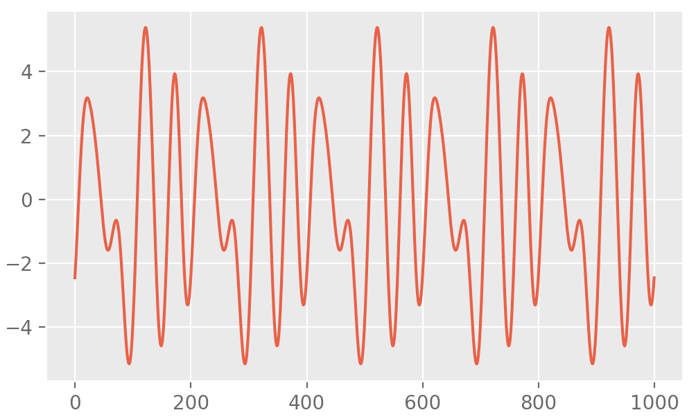
Fast Toeplitz Matrix-Vector Products and Solving
Circulant matrix-vector products can be fast due to the way circulant matrices can be decomposed using their fourier transforms. Toeplitz matrices can be ‘embedded’ into a circulant matrix and their matrix-vector products can be computed efficiently too.
Main reference:
J. Dongarra, P. Koev, and X. Li, “Matrix-Vector and Matrix-Matrix Multiplications”. In Z. Bai, J. Demmel, J. Dongarra, A. Ruhe, and H. van der Vorst, editors. “Templates for the Solution of Algebraic Eigenvalue Problems: A Practical Guide”. SIAM, Philadelphia, 2000. Available online.
This can then be used to compute multivariate normal log-densities quickly. Furthermore, this multiplication can then be used in conjugate gradient solvers to efficiently compute inverse-matrix-vector products in \(O(n \log n)\) time and \(O(n)\) space.
I’ve contributed a function to scipy - scipy.linalg.matmul_toeplitz that does this computation. The source can be viewed here.
Toeplitz matrices can be inverted in quadratic time using the Levinson algorithm, that also has the capability of returning a determinant as a side product using no more computation (as I understand).
Toeplitz Matrix Cholesky Decomposition
I got the toeplitz_cholesky library from here and compiled it (ctypes is used to load this into python). I believe that the following algorithm calculates the cholesky decomposition in \(O(n^2)\) time.
C/Python Code
# in bash: clang -shared -fpic toeplitz_cholesky.c -o tc.dylib -O3

import time
import numpy as np
import matplotlib.pyplot as plt

plt.style.use("ggplot"); plt.ion()

dll = np.ctypeslib.load_library("tc", ".")
np_poin = np.ctypeslib.ndpointer

def kernel(n = 100):
	k = np.linspace(0, 5, n)
	k = np.exp(-(k - k[0])**2)
	k[0] += 1e-10
	return k

def toep_chol_prepare(n):
	type_input_1 = np.ctypeslib.ctypes.c_int64
	type_input_2 = np_poin(dtype = np.double, ndim = 1, shape = n)
	type_output = np_poin(dtype = np.double, ndim = 2, shape = (n, n))

	dll.t_cholesky_lower.argtypes = [type_input_1, type_input_2]
	dll.t_cholesky_lower.restype = type_output
	return dll.t_cholesky_lower

def timer(n = 100):
	func_ptr = toep_chol_prepare(n)
	tic = time.time()
	L = func_ptr(n, kernel(n))
	toc = time.time()
	return toc - tic, L

if __name__ == "__main__":
	runtime, L = timer(10000) # half a second!
	x = np.matmul(L.T, np.random.normal(size = 10000))
	plt.plot(x)
	input("Press the enter key to quit.")
End
2021
Efficient Gaussian Process Computation
Using einsum for vectorizing matrix ops
Gaussian Processes in MGCV
I lay out the canonical GP interpretation of MGCV’s GAM parameters here. Prof. Wood updated the package with stationary GP smooths after a request. Running through the predict.gam source code in a debugger, the computation of predictions appears to be as follows:
Short Side Projects
Snowflake GP
Photogrammetry
I wanted to see how easy it was to do photogrammetry (create 3d models using photos) using PyTorch3D by Facebook AI Research.
Dead Code & Syntax Trees
This post was motivated by some R code that I came across (over a thousand lines of it) with a bunch of if-statements that were never called. I wanted an automatic way to get a minimal reproducing example of a test from this file. While reading about how to do this, I came across Dead Code Elimination, which kills unused and unreachable code and variables as an example.
2020
Astrophotography
I used to do a fair bit of astrophotography in university - it’s harder to find good skies now living in the city. Here are some of my old pictures. I’ve kept making rookie mistakes (too much ISO, not much exposure time, using a slow lens, bad stacking, …), for that I apologize!
Probabilistic PCA
I’ve been reading about PPCA, and this post summarizes my understanding of it. I took a lot of this from Pattern Recognition and Machine Learning by Bishop.
Spotify Data Exploration
The main objective of this post was just to write about my typical workflow and views. The structure of this data is also outside my immediate domain so I thought it’d be fun to write up a small diary working with the data.
Random Stuff
For dealing with road/city networks, refer to Geoff Boeing’s blog and his amazing python package OSMnx. Go to Shapely for manipulation of line segments and other objects in python, networkx for networks in python and igraph for networks in R.
Morphing with GPs
The main aim here was to morph space inside a square but such that the transformation preserves some kind of ordering of the points. I wanted to use it to generate some random graphs on a flat surface and introduce spatial deformation to make the graphs more interesting.
SEIR Models
The model is described on the Compartmental Models Wikipedia Page.
Speech Synthesis
The initial aim here was to model speech samples as realizations of a Gaussian process with some appropriate covariance function, by conditioning on the spectrogram. I fit a spectral mixture kernel to segments of audio data and concatenated the segments to obtain the full waveform.
Sparse Gaussian Process Example
Minimal Working Example
2019
An Ising-Like Model
… using Stan & HMC
Stochastic Bernoulli Probabilities
Consider: